PRY

What is PRY

PRY is a bio-economic livestock herd/population model developed by Dr. habil. Richard Baptist (formerly of the University of Nairobi and the University of Hohenheim) in 1988. PRY is a species independent, livestock-driven, herd model, which combines deterministic and stochastic procedures and allows for assessing herd/population productivity, simulating herd/population development, comparing productivity between livestock systems and management strategies within livestock systems.

PRY derives a productivity index (PI) "total output value/dry matter intake (TOV/DMI)" as a measure of overall productivity of an animal production system. Dry matter intake is chosen as denominator in this index because feed is considered the most limiting production asset as it generally accounts for the major part of production costs and is the main input factor in extensive animal husbandry systems.

PRY in its original DOS based version consists of six single components or modules (DIC, PIC, SAM, FOC, BOI, APE). Demographic input parameters are entered and stored in DIC. Produce-related input parameters are entered and stored in PIC. Deterministic modelling components SAM, FOC, and BOI derive population structure, numeric offtake, life expectancies and potential rate of increase of population for an infinitely large, closed equilibrium population (a population at steady state) from the DIC parameters. Total offtake value per dry matter intake for different disposal strategies is derived adding information from the PIC parameters, thus the model permits to find an optimal culling strategy (FOC). With a specific culling regime specified, a detailed breakdowns of offtake and intake (BOI) can be derived. The stochastic animal population emulator APE permits the simulation of herd/population development over time.

PRY was further developed by Dr. Richard Baptist into an MS Excel add-in named HerdLife. HerdLife combined the different modules above and eased handling of the model, particularly parameter input as well as display and storage routines.

In a current effort encouraged by the model author, PRY / HerdLife will be linked to external data sources – i.e. spreadsheet or database applications often used in research projects as well as livestock management programmes such as CowSense (TM by Midwest Microsystems). Thus, input parameters can be directly read/retrieved from data either routinely collected in commercial livestock operations or data generated by research projects. The initiative is carried forth by a consortium between Science Data Services (Dr. Simon Riedel), the German Institute for Tropical and Subtropical Agriculture [www.ditsl.org DITSL] (Dr. Christian Hülsebusch and Prof. Dr. Brigitte Kaufmann) and the University of Kassel (Dr. Uwe Richter, Prof. Dr. Eva Schlecht). The consortium appreciates the generous permission of the author, Dr. habil. Richard Baptist, to further develop his valuable tool with the aim to provide a flexible decision support tool for the management of livestock systems.

In a first step, the model was transcribed into a standalone application running under Windows XP/7 named PRY 3.0 beta – which can be downloaded here for test purposes

In a next step, a MySQL database will be coupled to PRY 3.0 beta that permits translation of CowSense (TM by Midwest Microsystems) export data into demographic input parameters for PRY.

DIC - Demographic Program Input Constants

Purpose of DIC

PRY provides an interactive routine for entering demographic parameters or inherent fitness traits. These are: survival rates, selective culling rates, age at first parturition, parturition interval and litter size. This routine is referred to as DIC (Demographic Program Input Constants). At every step of parameter entry, checks are carried out, error messages displayed and only consistent values accepted to avoid crashing of the simulation and derivation routines. Specification of age groups, rates and histograms is flexible. After entry, the parameters are formatted and saved to a work file from which they are later retrieved by the simulation and derivation routines.

Survival Rates

A survival rate is the fraction of animals still present at the end of a time interval if no living animal were disposed of. Such a rate represents an inherent potential and can be specified even for age classes which, in practice, are not at all represented because animals are culled before that age. Survival rates observed under a specific culling pattern may well differ from the survival rates to be specified as inherent demographic parameters. Survival rates can be specified for arbitrary age classes as either an annual rate or as a fraction surviving to the end of the specified interval. Such an interval or age class is defined in terms of a starting week or month of age and an ending week or month. The period covered can be more or less 8than a year.

Animals surviving to the ’biological’ maximum age specified, are assumed to be lost, rather than culled at the last time-step. However, animals surviving to a cull-for-age threshold lower than the ’biological’age limit,are assumed to be culled.

If only one survival rate per sex is specified, the age group then includes all ages from the first month or week of age up to the highest possible age. A maximum of 14 age groups can be defined. Male and female survival rates may be the same. However, age group boundaries and corresponding rates can also be defined for each sex separately.

Losses and culls in breeding females are not always clearly distinguishable. Emergency slaughter is an anticipated mortality or a cull, depending on the value of deadweight. Youngstock is never disposed of on voluntary grounds unless it has reached ’marketing’ age. Therefore, forced culls in youngstock are to be aggregated with losses. The value of deadweight can be adjusted correspondingly, to reflect an expected average of real losses of low salvage value and forced cullings of high salvage value.

SCRAPSelective culling rates in breeding females

In practice, breeding females which have not yet reached the cull-for-age threshold are not culled on a yearly basis as assumed in most livestock productivity models. Rather, a certain fraction per parity can be expected to fail to conceive or pose problems like low yield or poor health. Culls based on problems like low yield or conformation are not really forced ones like culls for failure-to-conceive or poor health. Both forced and arbitrary culls of breeding females do, however, have the same effect in terms of population dynamics. That is why they are treated alike and aggregated into a ’selective culling rate per parity’ of breeding females (SCRAP-rate). For example, if the ’true’ sterility rate is 0.05 and the rate of low yielders is 0.10, the SCRAP-rate to be entered would be 0.15, which is the rounded value of the conditional probability:

1–(1–0.10) (1–0.05) = 0.145

assuming that an animal’s yield level is independent of its reproductive performance.

The SCRAP-rate should not include the fraction of lost animals, i.e., forced culls with a low enough salvage value to be aggregated with mortalities. The distinction is often made between involuntary and voluntary culls. The best way to avoid confusion is probably to first think in terms of animal losses, on the one hand, and culls on the other. Then, culls are further differentiated according to whether they are forced or arbitrary. It depends on the context of the modelling exercise how ’exits’ are partitioned among these categories.

’Sterile’ breeding females are assumed to be recognized as such only when a parturition is overdue. In the case of ’sterile’ nulliparous breeding females this means that they are culled at an age when practically all ’fertile’ age-mates have given birth. In the case of ’sterile’ primi- and multiparous animals it means that they are culled when fertile age-mates have nearly all given birth again. Animals with a low yield and animals of poor health are, like ’steriles’ likely to be culled only after weaning or at the end of a lactation when the parturition interval, statistically speaking, tends towards its end. Therefore, selective culls, both for failure-to-conceive and other ’problems’, are treated alike and assumed to take place shortly before the next parturition is due.

In conclusion, the compound rate of selective culling per parity is to give the fraction of breeding females in an age group which are earmarked to be culled when a next (or the first) parturition is ’overdue’. When culling actually takes place is detailed in the sections on the animal population emulator and the stationary-state demographic model, respectively. Both routines use the same parameter of a SCRAP-rate. The SCRAP-rate gives a fraction per parity. However, age dependency is taken into account by varying the rate by age. A minimum of two age groups and a maximum of 14 can be defined. The SCRAP-rate of the first age group is applied to nulliparous breeding females. The other rates are applied to those breeding females having a parturition in the respective age group. Like survival rates, SCRAP-rates are inherent parameters. An ’ear-marked’ breeding female can die or reach the cull-for-age threshold before ’scrapping’ actually takes place towards the expected end of the parturition interval.

Age at first parturition

The age at first parturition is specified in weeks or months. It is given as a frequency distribution. The special case of a histogram with only one column represents a statistical population with a mean but zero variance. As the column heights of the histogram are edited, the mean and standard deviation are calculated and displayed by the program. The histogram can be composed of up to 14 columns. The height of each column is entered using an arbitrary scale. It is not essential but preferable to specify a histogram with more than one column. With only one column very fluctuating population sizes will result for the dynamic model due to an effect of synchronisation. A multi-column histogram, even if it is the very crude approximation of a rectangular distribution, will desynchronize births. Consequently, simulated population sizes and structures become more continuous.

Parturition interval

Like age at first parturition, the parturition interval is specified as a histogram. The remarks of the preceding paragraph concerning age at first parturition apply. The parturition interval represents only a partial aspect of reproductive fitness. In the model, it is complemented by the SCRAPrate which normally represents an age-dependent sterility rate.

Litter size

Litter size is specified as the histogram of number-of-young per litter. An average litter size which is not an integer number cannot be specified as a single-column histogram. A multiplecolumn histogram with integer class means must be defined so as to get an appropriate population mean. This weighted average is continuously updated and displayed as the histogram of litter size is edited. Even when average litter size can be given as an integer value, it is preferable to enter a multiple-column histogram, in order to smoothen fluctuations of population size in runs of the dynamic model.

Before you Start

Hardware Requirements

Hard and Software Requirements

System Architecture	This system runs on 32 and 64bit Systems
Operation System	Microsoft Windows
Win Version	Win 7, Win 8, Win 10
HDD Space required	300MB
RAM	2 GB (4 Recommended)
Misc	Requires the Installation of some Database-Modules from Microsoft

Download

Unless you are a developer or require Modules from the original DOS Software, you most proably want to use the 3.x Version of the Software, provided as an installable Windows App. Download of other Versions below

PRY 3.x

Latest Version

Version	File	ReleaseNotes
1.0.13	PRY 3.0.12 Windows Installer	abcdef.txt

Access previous Versions of PRY

• Version History
• Download PRY 2.x
• Download PRY 1.x

Installation Manual

Requirements
What	Description
PRY Installer	Get the PRY Zip File (here)
Unzip Software	WinRar, WinZip or 7zip - you most probably have such Software on your computer

1.) Extract the Zip File into any Folder

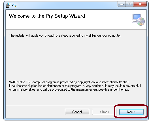
2.) Open the Folder and click on "Setup.exe"

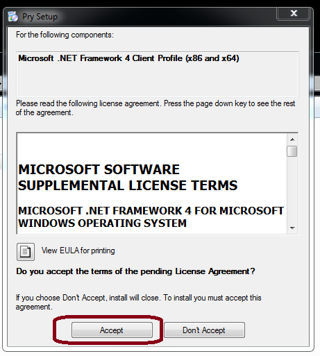
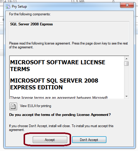
3.) Two modules will be directly downloaded from Microsoft - if you don't already have them installed on your computer, you need to agree to the Terms and Conditions and follow the installation instructions of those modules

4.Allow Microsoft to install Modules on your Computer

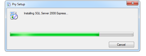
5. The installation is in process

PRY' is now successfully installed on your Computer. You will find a Link to the Software on your Desktop (Icon is black, so you might not see it directly when your Background is black) and in the Start-Menue.

If you encounter any problem with installing PRY on your computer, you may ask for support

User Manual

For other Versions see User Guide here

Version 2.x

PRY realized as Modules in an Excel sheet

Version 1.x

The original PRY, a DOS console Program

Model Input Parameters

Age at first Parturition

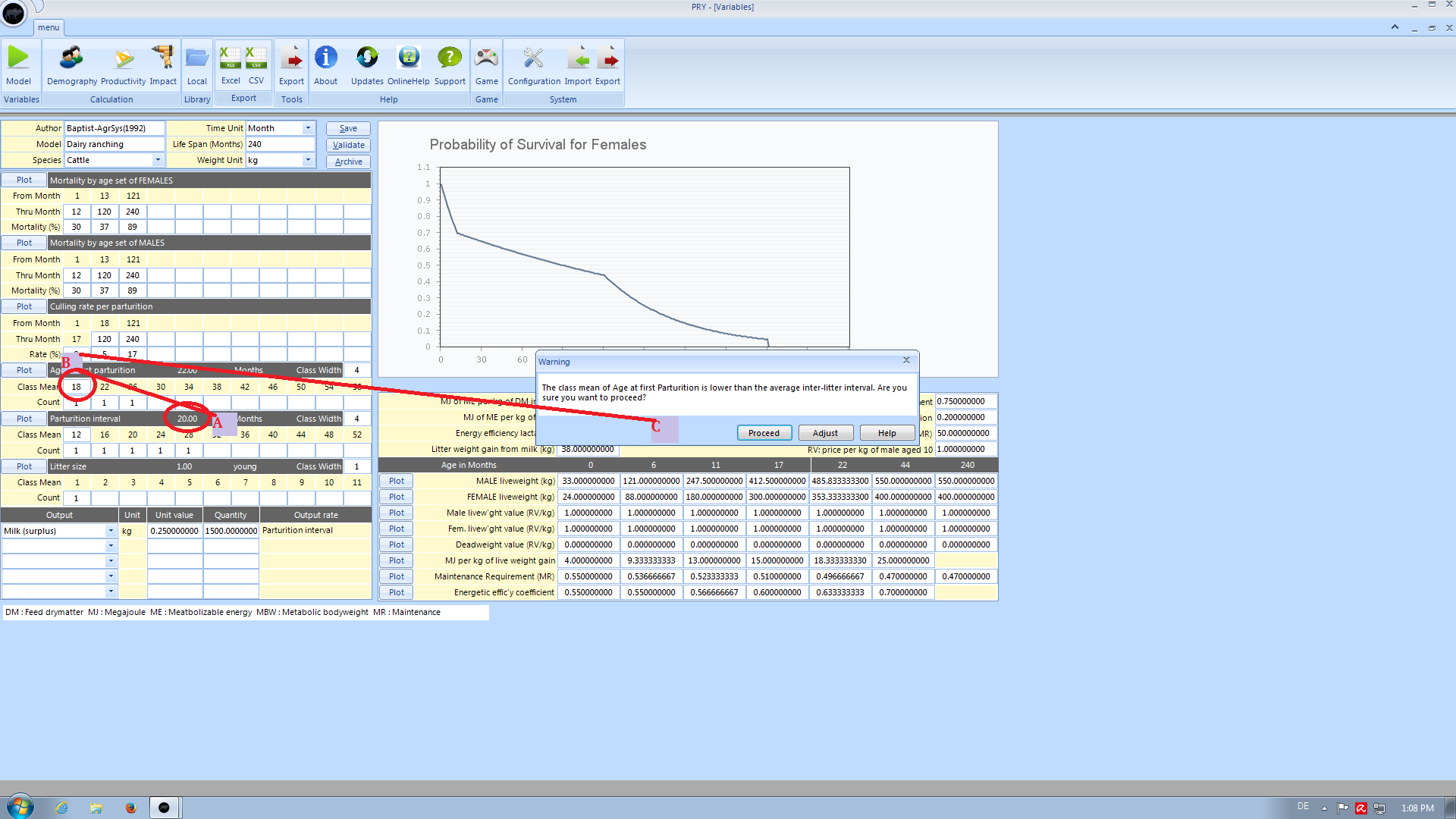
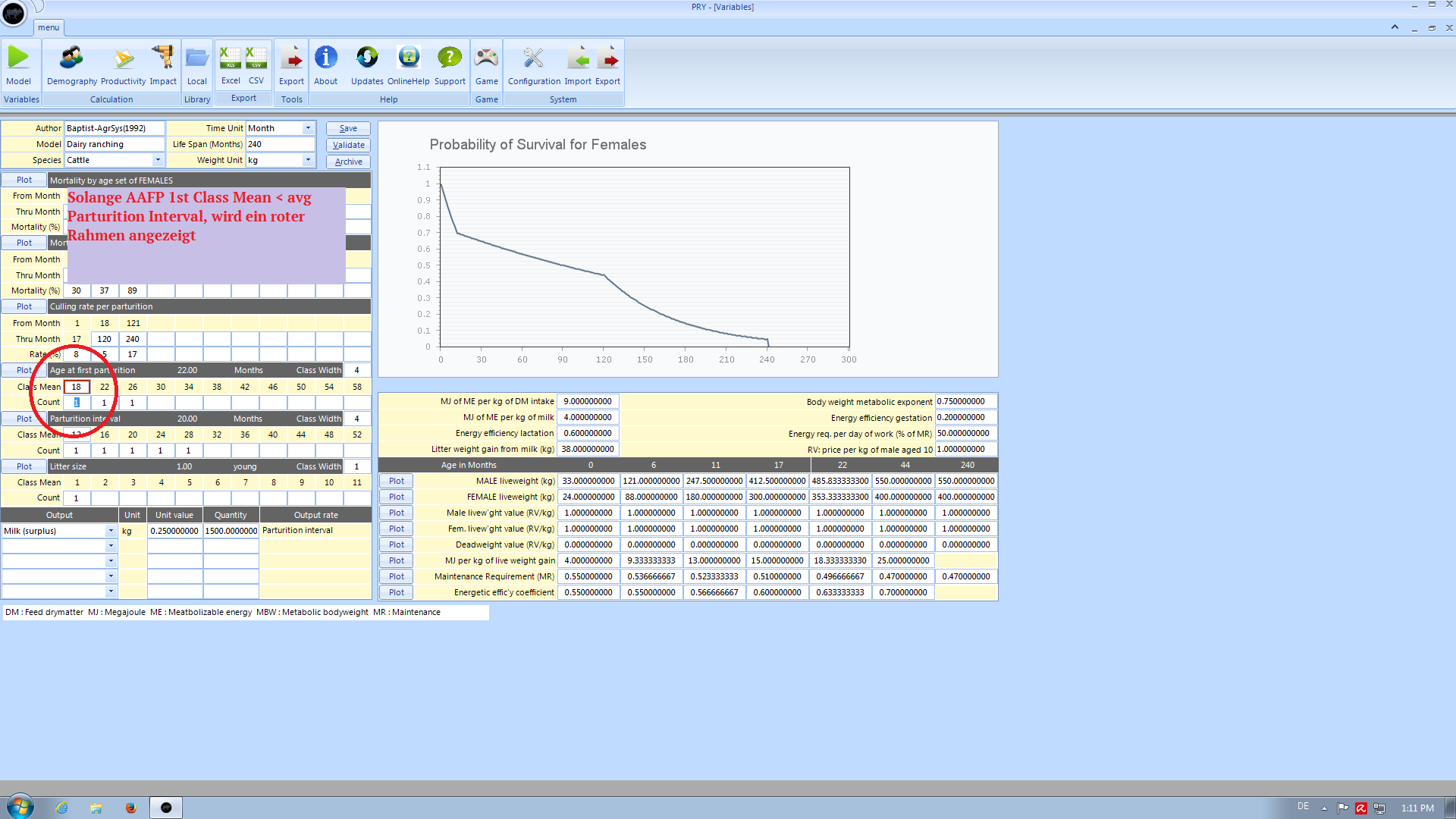
When a class mean in the first class of age at first parturition is entered which is below the average inter-litter interval, a warning shows up to recheck your values. You have three options:

• Proceed and leave your input as it is
• Correct your value
• Click the Help Button to learn why this value might be critical for your model

Literature

Many studies have been conducted by using the PRY Software. We are trying to collect all, so if you know of any further study, let us know, we will list them here. If you have any questions about those publications, you may contact DITSL , visit the [contact] page for further details.

Herd Analysis with PRY

Author	Year	Journal	Title	Link/File	Species
Baptist,R. Sommerlatte	1992	Small Ruminant Research	Evaluation of cropping strategies in game ranching using a livestock productivity model	http://dx.doi.org/10.1016/0921-4488(91)90124-9	Game
Fink H. and Baptist R.	1992	Better feeding for improved production - FAO Series	Herd dynamics modelling applied to a venison ranch in Kenya	http://www.fao.org/docrep/u8750t/u8750T04.htm	Game
Anonymous	1995	Wildlife and Nature	Herd Dynamics modelling applied to a Venison ranch in Kenya	PDF	Game
Fink	1990	unpublished (Diploma Thesis)	Schätzung demographischer Parameter in der Wildnutzung aus ermitteltem Propulationswachstum und -struktur, Entnahmerate und Zusammensetzung der Entnahme auf einer kenyanischen Wildranch	DOI	Game
Kaufmann, B.	199x			contact	Cattle/Camel
Huelsebusch, C.	199x			contact	Cattle/Camel
Dos Santos / Neuzling, A.	200x			contact	Cattle
Dickhoefer et al.	2012	Agricultural Systems 110,C, 131-141	Modeling herd development and revenues from Jabal Akhdar goats under current and intensified management	http://www.sciencedirect.com/science/article/pii/S0308521X12000583	Goat
Riedel et al.	2014	Livestock Science, 160, 151-162	The productivity of traditional smallholder pig production and possible improvement strategies in Xishuangbanna, South Western China	http://www.livestockscience.com/article/S1871-1413%2813%2900502-7/abstract	Pigs
Hofsommer	2014			contact	Cattle
Aufderheide, M.	2014			contact	Cattle
Wario, H.T.	2015	Social Ecological Research Series	An integrated assessment of resource use strategies in the Borana pastoral system of southern Ethiopia	http://d-nb.info/1075658810/34	Cattle

Methodology

Author	Year	Journal	Title	Link/File
Baptist, R.	1987	Agricultural Systems	Computer Simulation of Monitoring Herd Productivity under extensive Conditions: Sampling Error of Herd Size and Offtake Rate	http://dx.doi.org/10.1016/0308-521X(87)90003-5
Baptist, R.	1988	Agricultural Systems	Herd Flock Productivity Assessment using the Standard Offtake and the Demogram	http://dx.doi.org/10.1016/0308-521X(88)90022-4
Baptist, R.	1991	unpublished	PRY Manual	PDF
Baptist, R.	1992	Habilitation	Population Dynamics and Productivity at the stationary State of Culling Regimes in Livestock Herds and Flocks	PDF
Pittroff and Cartwright	2002	Arch. Latinoam. Prod. Anim.	Modeling livestock systems. I. A descriptive formalism	http://www.alpa.org.ve/PDF/Arch%2010-3/Archivos10(3)193.pdf
Rushton, J.	2009	CABI Publishing	The Economics of Animal Health and Production , p. 96	ISBN 1845931947